InReach
The InReach model computes accessibility indicators for zones, which represent how accessible different types of destinations are. For example, it can be used to assess how many jobs, shopping facilities and schools are accessible while residing in a specific zone. This indicator can be provided for several population groups. The indicator is primarily derived from Integrale Mobiliteitsanalyse (IMA).
Overview of computation steps
The computation of the indicator consists of two steps:
- Derivation of travel time decay curves, representing the 'acceptable' travel time for a certain group.
- Compute number of accessible destinations per zone, based on the computed curves.
For both steps a high-level intuitive explanation is provided in the sections below.
Travel time decay curves
A travel time decay curve can be used to represent how many trips experience a certain travel time, as illustrated in the figure below. For example, 100 percent of the trips experienced a travel time of >1 minute, 80 percent of the trips experience a travel time of >20 minutes, and 20 percent of the trips experience a travel time of >120 minutes. These numbers are illustrative.
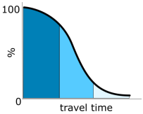
By assuming that the experienced travel time is equal to the acceptable travel time, one can derive that e.g. for 80 percent of the trips it is acceptable to travel for >20 minutes. The curves may be estimates from data, such as the Onderzoek Onderweg in Nederland conducted by Statistics Netherlands.
Computation of the indicator
The indicator aims to compute the potential number of e.g. jobs that can be reached within an acceptable travel time. We explain this intuitively based on the figure shown below. It depicts a zone, and the locations of jobs in the vicinity. The colors of the circles represent the decay curve values. For example, the dark blue circle represents the locations that are reachable within a given travel time, consistent with the colors in the curve from the previous section.
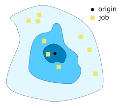
The number of jobs accessible within an acceptable time can subsequently be estimated by computing \(\int_{0}^{\infty} N_{jobs}(t) \cdot {TT}_{frac}(t)~ \,dt\), in which \(N_{jobs}\) denotes the number of jobs and \({TT}_{frac}(t)\) denotes the fraction of trips having a travel time \(\geq t\), which follows from the decay curve and it acts as a weight. Intuitively, jobs close to the zone are included in the computation with a high weight, while the weight associated with jobs far away approaches zero.
Input collections
In the overview below we show which data collections should be filled when running the model.
| Collection | Description |
|---|---|
| ir_activities | Information about the activity types. |
| ir_groups | Information about the population groups. |
| ir_zonal_activity_data | Information about the zonal activity. |
| ir_modalsplit_weights | Information about the modal split weights within a minimum and a maximum percentage value for combinations of activity_id and dimension_id. |
| ir_traveltime_weights | Information about the travel time weights within a minimum and a maximum time range value for combinations of activity_id, dimension_id and group_id (optional). |
| ir_urbandegree_weights | Information about the underdegree and weight per activity_id. |
| ir_group_percentage_per_zone | Information about group percentage values per group_id and zone_id. |
Output data
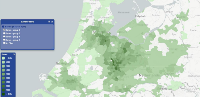
The output of the computation is available in the collection ir_basic_district_indicators, containing the indicator values. However, it is important to note that it is more intuitive to visualize them on the map, as illustrated below.
Parameters and settings
| Parameter name | Description | Type | Unit |
|---|---|---|---|
| processed_dimensions | Comma-separated list of dimension IDs that will be processed by the module | string | - |
| travel_time_thresholds | Comma-separated list of travel time thresholds; The thresholds correspond to the dimensions specified in processed_dimensions; Note that the thresholds only apply to the basic-district indicator |
string | hours |
| processed_group_ids | Comma-separated list of group IDs that will be processed by the module | string | - |
| IMA_indicator | If enabled, IMA indicators are computed | boolean | - |
| basic_district_indicator | If enabled, basic-district indicators are computed | boolean | - |
Sample Parameter JSON
[{"Name":"IMA_indicator","Value":true,"Type":3},{"Name":"basic_district_indicator","Value":false,"Type":3,"Unit":""},{"Name":"processed_dimensions","Value":"1,4,7","Unit":"comma-separated list"},{"Name":"travel_time_thresholds","Value":"100,100,100","Unit":"comma-separated list"},{"Name":"processed_group_ids","Value":"1,2","Unit":"comma-separated list"}]
Validation
The validation of the indicator mainly relates to the estimation process of the travel time decay curves from the data. During this process it is important to assess the quality of the fit given the data, based on e.g. the root mean squared error. Once this process has been conducted by a scientist, the model itself does not require further validation. It is important to note that all current applications of this model focus on the Dutch context, because of the availability of the data.
Literature
More details and related information can be found in the following references:
-
Goudappel. (2021). Achtergrondrapportage Integrale Mobiliteitsanalyse, ontwikkeling mobiliteit, stedelijke bereikbaarheid en. Rijkswaterstaat WVL.
-
Martínez, L. M., & Viegas, J. M. (2013, January). A new approach to modelling distance-decay functions for accessibility assessment in transport studies. Journal of Transport Geography, 26, 87-96. doi:https://doi.org/10.1016/j.jtrangeo.2012.08.018