Traffic Assignment

Traffic plays a central role in the functioning of cities, affecting accessibility, travel times, economic activity, environmental impacts, and the quality of urban life. The way vehicles move through a road network determines where congestion occurs, how efficiently people and goods can travel, and how infrastructure investments or policy measures influence mobility patterns.

The Traffic Assignment model calculates the route choice for all road-bound trips through the road network, using Dijkstra algorithm to find each trip's shortest path and iterating toward an equilibrium through deterministic multi-user-class assignment.

The model enables to interactively evaluate the impact of infrastructure and policy changes, such as modifications to road speed, capacity, or pricing. By simulating the resulting route choices of different vehicle types, including cars, trucks, and cyclists, the model helps assess how network changes affect traffic patterns and accessibility.

Macroscopic trip based model

The module is trip-based, meaning it simulates trips, and not individual travelers. In this way, a car trip can be for example an individual driving to work or a family of four traveling to the beach. Both situations are described by a single trip.

Controls

The model responds to the following interventions (controls):

Road speed

Adjust the mode-specific speed on a link.
Road capacity

Adjust the mode-specific capacity on a link.
Junctions

Alter junction specifications on the network.
Road closure

Close roads for certain modes.
Toll pricing

Set mode-specific pricing on a link.
New roads

Draw new network links and nodes.

Controls are configured in the main collection controltype, the default set for the Traffic Assignment model consists of:

ICON	JSON	NAME	OBJECT_ID	OBJECT_TYPE
road-control	[{"name":"SPEED_L","type":"text","label":"SPEED_L","default":"","validate":""},{"name":"SPEED_R","type":"text","label":"SPEED_R","default":"","validate":""},{"name":"CAPACITY_L","type":"text","label":"CAPACITY_L","default":"","validate":""},{"name":"CAPACITY_R","type":"text","label":"CAPACITY_R","default":"","validate":""}]	Speed & Capacity	1	road
turn-control	[{"name":"TURNDELAY","type":"text","label":"Turn delay","default":"999","validate":""}]	Close turn	15	turn_private
node-control	[{"name":"JUNCTIONTYPE","type":"select","label":"JUNCTIONTYPE","default":"","validate":"","options":[{"name":"1 - Equal priority","value":"1"},{"name":"2 - Give Way","value":"2"},{"name":"3 - Signalized","value":"3"},{"name":"4 - Roundabout","value":"4"},{"name":"5 - Roundabout + Signals","value":"5"},{"name":"6 - All Entry Stop","value":"6"}]}]	Junction type	2	node

Parameters

Parameters can be set trough the McControl and StoreEditor.

Parameter	Description	Default value
referenceRun	Write all matrix results to the reference columns and shut down the model	false
writeSkims	Write traveltimes, distances (and costs if monetaryCosts is set) to the ODMatrices of the defined dimensions	true
iterationsVolumeAveraging	The number of iterations if VolumeAveraging is used	false
dimensionsVA	A list of dimensions which should be assigned using volume averaging
dimensionsAON	A list of dimensions which should be assigned using All or Nothing assignment
sumDimensions	Dimensions fow which the intensities should be summed into a single "Derived Intensity" during the calculation
totalLoadDimension	The dimension to which the sumDimension "Derived Intensity" should be written
filterUTurns	Leave out all U-Turns when reading in the network	true
includeMonetaryCosts	Include monetary link costs in the path costs for assignments	false
availableGPUMemory	Maximum amount of GPU memory claimed by model	15
iterationsLUCE	Number of iterations if Luce is used	1
interpolationMethodLUCE	Interpolation method for Luce if used	0
AssignmentMethod	Assignment method (0 = VA, 1 = LUCE, 2 = STAVAQ)	0

Data collections

Data collections from the base bin:

Collection overviewtraf_dimensionsroadsroad_analysistraf_modestraf_nodestraf_turnstraf_zones

Collection	Description	Bin
traf_dimensions	The combination of travel mode, time of day and motive is called a dimension	Base
roads	The network to assign the different dimensions	Scenario
roads_analysis	Corrosponding links and OD pairs for the selected link analysis	Scenario
traf_modes	The nodes of the network	Scenario
traf_nodes	The nodes of the network	Scenario
traf_turns	The turns of the network	Scenario
traf_zones	The origin and destinations used in the OD-matrix	Scenario

Field	Schema	Description	Subscription
COST_DISTANCE	double	The costs for distance traveled	Read
COST_TIME	double	The costs for time traveled	Read
DAYPART	string	The name of the daypart	Read
DAYPART_ID	int32	The ID of the daypart	Read
DETAILS	string	Description of the dimension	Read
EXTRA	string	For notes about the dimension	Read
MODE_ID	int32	ID of the mode from traf_modes	Read
MOTIVE	string	Description of the travel motive	Read
OBKECT_ID	int32	Unique ID of the dimension	Read
PCU	double	The Personal Car Unit of the dimension	Read

Field	Schema	Description
A_L	double	BPR-A
A_R	double	BPR-A
B_L	double	BPR-B
B_R	double	BPR-B
C_L	double	BPR3-C
C_R	double	BPR3-C
CALCULATION_AREA	int32	Indicate if it is used in emission calculations (1)
CAPACITY_L	double	Capacity
CAPACITY_R	double	Capacity
CONSTRUCTION_TYPE	int32	Construction type (6=tunnel)
COST_L	double	Total toll for the link
COST_R	double	Total toll for the link
CREATED	double	Date created
D_L	double	BPR3-D
D_R	double	BPR3-D
DIMENSION_ID	int32	Dimension ID
DISTRICT_ID	int32	District (or sector) the road is in
E_BAP	double	Calculated emissions for link
E_BENZEEN	double	Calculated emissions for link
E_CO	double	Calculated emissions for link
E_CO2	double	Calculated emissions for link
E_EC	double	Calculated emissions for link
E_NH3	double	Calculated emissions for link
E_NO2	double	Calculated emissions for link
E_NOX	double	Calculated emissions for link
E_O3	double	Calculated emissions for link
E_PM10	double	Calculated emissions for link
E_PM25	double	Calculated emissions for link
E_SO2	double	Calculated emissions for link
FNODE_	int32	From or A-node
IC_RATIO_L	double	Calculated IC ratio for mode
IC_RATIO_R	double	Calculated IC ratio for mode
INTENSITY	double	Calculated flow (L+R combined)
INTENSITY_L	double	Calculated flow
INTENSITY_R	double	Calculated flow
LANE_COUNT_L	int32	Number of lanes
LANE_COUNT_R	int32	Number of lanes
LENGTH	double	Length in m
LINKTYPE_L	int32	Link type
LINKTYPE_R	int32	Link type
OBJECT_ID	int32	Road ID
PCBUA	double	Buses evening
PCBUD	double	Buses day
PCBUN	double	Buses night
PCLIA	double	Light traffic evening
PCLID	double	Light traffic day
PCLIN	double	Light traffic night
PCMOA	double	Medium traffic evening
PCMOD	double	Medium traffic day
PCMON	double	Medium traffic night
PCMZA	double	Medium heavy traffic evening
PCMZD	double	Medium heavy traffic day
PCMZN	double	Medium heavy traffic night
PCUURA	double	PCU traffic evening
PCUURD	double	PCU traffic day
PCUURN	double	PCU traffic night
PCZWA	double	Heavy traffic evening
PCZWD	double	Heavy traffic day
PCZWN	double	Heavy traffic night
SHAPE	complex:geometry	Geometry
SPEED_L	double	Model speed
SPEED_R	double	Model speed
TNODE_	int32	To or B-node
TRAVEL_CAP_L	double	Calculated capacity (STAVAQ)
TRAVEL_CAP_R	double	Calculated capacity (STAVAQ)
TRAVEL_SPEED_L	double	Calculated speed
TRAVEL_SPEED_R	double	Calculated speed
TRAVEL_TIME_L	double	Calculated travel time
TRAVEL_TIME_R	double	Calculated travel time
TREECODE	int32	Tree code (0, 0.5, 1) for AIR
WEGDEK_COD	int32	Surface type for NOISE

Field	Schema	Description
ANALYZED_OBJECT_ID	int32	Selected link object ID
DIMENSION_ID	int32	Selected link dimension ID
INTENSITY_L	double	Intensity on link
INTENSITY_R	double	Intensity on link
OBJECT_ID	int32	Object ID of link
RELATIVE_INTENSITY_L	double	Intensity relative to selected link
RELATIVE_INTENSITY_R	double	Intensity relative to selected link
SHAPE	complex:geometry	Geometry
WIDTH_L	double	Width
WIDTH_R	double	Width

Field	Schema	Description	Subscription
DESCRIPTION	string	Name of the mode
OBJECT_ID	int32	Unique object id

Field	Schema	Description
OBJECT_ID	int32	Unique object ID
X	double	X-coordinate
Y	double	Y-coordinate

Field	Schema	Description
A	double	BPR-A
B	double	BPR-B
CALIBRATION_FACTOR	double	Factor to reduce turn delay
CAPACITY_IN	double	Input capacity
CREATED	double	Date created
CYCLE_TIME	double	Cycle time for VRI
DIMENSION_ID	int32	Dimension id
GREEN_OFFSET	double	Offset for green time
GREEN_TIME	double	Green time
INTENSITY	double	Calculated intensity
NODE_A	int32	From node
NODE_A_X	double	Coordinate
NODE_A_Y	double	Coordinate
NODE_B	int32	Via node (junction ID)
NODE_B_X	double	Coordinate
NODE_B_Y	double	Coordinate
NODE_C	int32	To node
NODE_C_X	double	Coordinate
NODE_C_Y	double	Coordinate
OBJECT_ID	int32	Object ID
TURNDELAY	double	Calculated turn delay
TURNDELAY_IN	double	Static turn delay input
TURNTYPE_ID	int32	Turn type

Field	Schema	Description
ARRIVALS	double	Attraction
CREATED	double	Create date
DEPARTS	double	Production
DISTRICT_ID	int32	Corresponding district
NAME	string	Name of the zone
OBJECT_ID	int32	Unique object ID
SHAPE	complex:geometry	Geometry
X_CENTROID	double	Centroid X
Y_CENTROID	double	Centroid Y

Data requirements

The calculation model requires the following data:

Dataset	Description	Common source	Importance
OD-matrices	The trips from- and to every origin- destination zone.	Conventional traffic model such as Visum, OmniTRANS or Emme.	Required
Network	Nodes and edges of the network to assign to, including properties such as speed and capacity.	Conventional traffic model.	Required
Skim-matrices	The traveltime and distance between every origin- destination zone.	Conventional traffic model.	Optional
Population	Charecteristics such as the distribution of age, car ownership and income for every origin- destination zone.	Statistical departement	Optional
Parking	Information about parking capacity and pricing for every origin- destination zone.	Parking departement	Optional
Toll	Information on pricing for roadways.	Road authority	Optional

Methodology

The assignment utilizes a static deterministic multi-user-class (equilibrium) assignment and allows to assign modes trough an all-or-nothing and/or volume averaging assignment technique. The all-or-nothing technique assigns traffic between an OD-pair on the shortest path. The volume averaging technique (re)assigns traffic during multiple iterations, with this technique the impact of congestion on route choice is taken into account.

The goal of static traffic assignment is to allocate a given travel demand (a set of trips with fixed origins and destinations) on the transportation network in order to obtain an initial spatial distribution of the traffic volume. Static assignment assumes that the number of trips on a link will be constant during the considered period of time and that all trips will be completed during this period. The resulting traffic volume represents the average conditions for the time period under consideration, making the technique suitable for studying specific periods such as the morning peak hours or an average weekday. A limitation of static assignment is its inability to fully capture dynamics of trip departure and real-time routing behavior with the risks of underestimating congestion levels. In addition, static assignment may result in link volume that exceeds link capacity. In spite of these limitations, static assignment is a valuable approach to traffic analysis as it allows to quickly estimate the use of traffic networks and to develop an initial appreciation of the situation.

The following methods are used within the TrafficAssignment model:

1. BPR function
To determine the travel times between origins and destinations.

2. Dijkstra's algorithm
To determine the shortest path between origins and destinations.

3. All-or-nothing and volume averaging assignment methods
To assign trips to the network.

Travel time function

For computing link travel times Urban Strategy uses the BPR function, which is developed by the American Bureau of Public Roads. It defines the relationship between travel time, volume and capacity in accordance with the following formula:

\[ T = T_0 \cdot \left( 1 + \alpha \left( \frac{I}{C} \right)^\beta \right) \]

where:

\(T\) is the travel time
\(I\) is the intensity
\(C\) is the capacity
\(T_0\) is the free-flow travel time
\(\alpha\) and \(\beta\) are user-defined coefficients

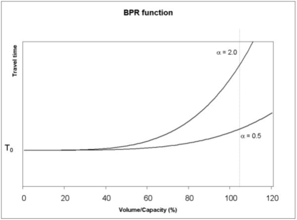
The relationship is as shown in the figure below. In short, \(T_0\) represents a base travel time which is then factored to give a new travel time for a given link. If \(\alpha = 0.5\), delays will occur if the link volume is approaching full capacity (main highways). If \(\alpha = 2.0\), significant delays will occur well before full capacity is reached (residential roads) as shown in the figure below. The function is assumed to simulate the delay occurred in a roadway as a consequence of intensity approaching the road capacity.

Dijkstra's algorithm

Urban Strategy computes shortest paths from a given origin \(S\) using Dijkstra's algorithm (forward search): the length (cost) of a link between A and B in the network is denoted by \(d_{A,B}\). The path or route is defined by a series of connected nodes, A-C-D-H, etc., whilst the length of the path is the arithmetic sum of the corresponding link lengths in the path. Let \(d_A\) denote the minimum distance from the origin of the tree to the node or centroid \(A\); \(P_A\) is the predecessor or backnode of \(A\) so that the link \((P_A, A)\) is part of the shortest path from \(S\) to \(A\). The procedure for building a minimum path tree from \(S\) to all other nodes is described as follows:

Initialization: Set all \(d_A = \infty\) (a suitable large number depending on computer and compiler) except \(d_S\) which is set equal to 0; set up a loose-end table \(L\) to contain nodes already reached by the algorithm but not fully explored as predecessors for further nodes. They are the tip of the tree as branches grow to reach all nodes. Initialize all entries \(L_i\) in \(L\) to zero, and all \(P_A\) to a suitable default value.

Procedure starting with the origin \(S\) as the ‘current’ node is \(A\):

Examine each link \((A, B)\) from the current node \(A\) in turn and, if \(d_A + d_{A,B} < d_B\) then set a new value for \(d_B = d_A + d_{A, B}\), make \(P_B = A\) and add \(B\) to \(L\);
Remove \(A\) from \(L\), if the loose-end table is empty, stop; otherwise,
Select another node from the loose-end table and return to step 1 with it as the current node.

Three comments should be made at this stage. First, routes are in general not allowed to use centroids; therefore in step 1, \(B\) would not be added to \(L\) if it was a centroid. Second, Dijkstra selects the node nearest to the origin, i.e. the node \(L_i\) such that \(d_{L_i}\) is a minimum. This requires some additional calculations (including sorting of nodes using a priority queue) but ensures that each link is examined once and only once. Finally, trees are stored in the computer as a set of ordered backnodes in which \(A\) is the backnode of \(B\) if link \((A, B)\) forms part of the tree.

The shortest route can be determined on the basis of either distance or travel time (including turn delays). Urban Strategy converts these attributes into a generalized cost according to pre-defined weighting factors. It should be noted that in a simple assignment such as all-or-nothing (discussed below), the travel time is a function of distance and travel speed. However, while accounting for congestion, the travel time becomes a function of the I/C ratio, defined by the BPR function.

The basic generalized cost formulation is best summarized by the following equation:

\[ G = \lambda \cdot D + \mu \cdot T \]

where:

\(G\) is the generalized cost
\(D\) is the travel distance
\(T\) is the travel time. This includes static turn delays. In a volume averaging assignment (discussed below) the travel time is determined by the BPR function
\(\lambda\) is the coefficient for distance applied throughout the network
\(\mu\) is the coefficient for time applied throughout the network

Paths built using this Generalized Cost formulation with or without capacity effects are called deterministic as opposed to stochastic (randomized). Urban Strategy does not account stochastic effects in the generalized cost, and thereby in route choice.

Traffic assignment methods

Having built the shortest paths in the network, there are various ways as how the trips can be assigned (loaded) to the network. There is the 'all-or-nothing' assignment which ignores the effects of congestion using just the shortest paths. Volume averaging is a path based method that iteratively assigns the current shortest path taking congestion effects into account. The local-user cost equilibrium method is an origin or bush based algorithm assigning multiple paths towards a single destination in one iteration, hence needing more memory but converging in fewer iterations.

All-or-Nothing (AON)

This assumes that all trips between an origin and a destination take the shortest path as determined by the generalized cost. It also assumes that there are no capacity problems and that this path is perceived by everyone as the shortest path. There are no iterations required.

Volume Averaging (VA)

This assumes that link flows are influenced by existing link flows (hence travel times) and are affected by link capacity. This requires an iterative process by which trips are loaded onto the network and where link travel times are adjusted according to the assignment volume and capacity using a Travel Time Function (BPR function). The objective is to achieve a network wide balance, or equilibrium, between link flows and link speeds (times), taking into account the network capacity. Trips can be loaded onto the network using a volume averaging approach.

In a volume-averaging assignment, also known as the method of successive averages, volumes (demand) are assigned to a network in an iterative process. In the traffic model, the first step in the iteration is always an AON assignment on the shortest route for the demand. The summing of the traffic volumes in the first steps is assumed to simulate the network characteristics of a pre-load situation in the road, including freight, car traffic, etc.

Volume is calculated as a linear combination of the volume found in the previous iteration and the volume added by means of an all-or-nothing assignment performed in the current iteration. By default, in each iteration of a volume-averaging assignment, the fraction \(1/n\) is used to increase the link volume and the value \((1-1/n)\) to reduce it, \(n\) being the number of iterations.

The volume averaging process terminates either when convergence has been detected i.e. when the maximum number of iterations \(N\) has been reached. The number of iterations is user-defined. Effectively when the convergence criteria is reached, we can conclude to a degree of certainty that traffic has achieved a Deterministic User Equilibrium (DUE).

The Volume Averaging method uses the Relative Gap as stopping criterion. When this value is below the threshold, which is usually defined as a small, non-zero value, the assignment will be considered as converged and the assignment will be stopped. The formula for the gap is as provided below:

\[ DG^i = \frac{\sum_a c_a x_a}{\sum_{rs} \pi_{rs}d_{rs} } -1 \]

where:

\(DG^i\) is the duality gap value for iteration \(i\)
\(c_a\) is the cost of link \(a\)
\(x_a\) is the load on link \(a\)
\(\pi_{rs}\) is the optimal cost from \(r\) to \(s\)
\(d_{rs}\) is the demand from \(r\) to \(s\)

The gap \(DG^i\) refers to the flow-weighted difference between current total cost estimates on the network, as determined by the present flow pattern and the speed/flow curves, and the costs if all traffic would use minimum cost routes (as calculated by the next all-or-nothing assignment).

Local-User Cost Equilibrium (LUCE)

The LUCE algorithm is an origin or bush based algorithm which uses an all or nothing assignment as starting point. For each destination, a directed acyclic graph (the bush) is used to assign the trips from all other zones via multiple paths at once to a destination. The bushes are checked and updated every iteration. Moreover, the trips are updated every iteration using a quadratic linear interpolation method per destination.

The LUCE method enables the assignment to spread the trips at multiple paths in a single iteration. This can make the model converge in fewer iterations than e.g. VA. However, this comes at the cost of more memory being used (storing all assigned trips per zone) and the iterations being slower. Hence, a trade off can be made.

Performance benchmark

Calculation times of the TrafficAssignment model with different datasets and iterations.

Setup	Zones	Links per mode	Modes	Iterations: 5	Iterations: 10	Iterations: 20	Iterations: 30
San Diego County	4.947	42.738	3	00:31,9	00:39,7	00:53,7	01:08,6
Amsterdam city	3.035	39.007	3	00:11,4	00:12,9	00:19,5	00:28,9
Amsterdam region	5.460	108.079	3	00:33,0	00:40,9	00:59,1	01:17,4
The Netherlands (National Model System (LMS))	1.565	112.860	3	00:26,3	00:42,2	01:12,5	01:42,0
Eindhoven Metro*	6.275	174.508	3	00:49,0	01:08,2	01:50,5	02:29,9

*Eindhoven Metro ran with limited memory capacity (24GB). Using sufficient memory capacity (ca. 80GB) would lead to about 1/3 of the documented calculation time.